Writing a custom implementation

New in version 0.2

In every operation and functional in xitorch, there are a few method implementations are available (e.g. solve_ivp() has "rk34", "rk45", etc). What if those implementations are not good enough for you? The answer is: just write your own, and you can still take the advantage of higher order differentability provided by xitorch.

For xitorch functionals (i.e. functions that take functions as inputs, such as rootfinder, quad, etc), the custom implementation will run in torch.no_grad() environment, so you don’t have to worry about in-place operations, backward instability, etc in your implementation. You can also use non-PyTorch or even non-Python implementation (with appropriate wrapper). This does not apply for operations, such as Interp1D and SQuad, where the gradient is obtained via backward calculation of the implementation.

To write a custom implementation of a method, it must follow the signature of the functional or operation without bck_options and method arguments. For example, the signature of solve_ivp() is

solve_ivp(fcn, ts, y0, params, bck_options, method, **fwd_options)

so the signature of your custom implementation should be

my_solve_ivp_impl(fcn, ts, y0, params, **fwd_options)

Let’s take an example of writing the forward Euler step in solve_ivp(). The forward Euler step is simply given by

\[\mathbf{y}_{i+1} = \mathbf{y}_i + \mathbf{f}(t_i, \mathbf{y}) (t_{i+1} - t_i).\]

The forward Euler can be implemented as below

import torch
import matplotlib.pyplot as plt
from xitorch.integrate import solve_ivp

def euler_forward(fcn, ts, y0, params, verbose=False, **unused):
    with torch.no_grad():
        yt = torch.empty((len(ts), *y0.shape), dtype=y0.dtype, device=y0.device)
        yt[0] = y0
        for i in range(len(ts)-1):
            yt[i+1] = yt[i] + (ts[i+1] - ts[i]) * fcn(ts[i], yt[i], *params)
        if verbose:
            print("Done")
        return yt

I use torch.no_grad() above just to illustrate that the gradient propagation is not needed in the custom implementation. In the example above, all the required arguments are present (i.e. fcn, ts, y0, params) plus one additional option for the implementation (i.e. verbose). The additional options must have a default value to comply with other implementations.

Now, using the above implementation is straightforward, just put the function above as input to the method argument in solve_ivp().

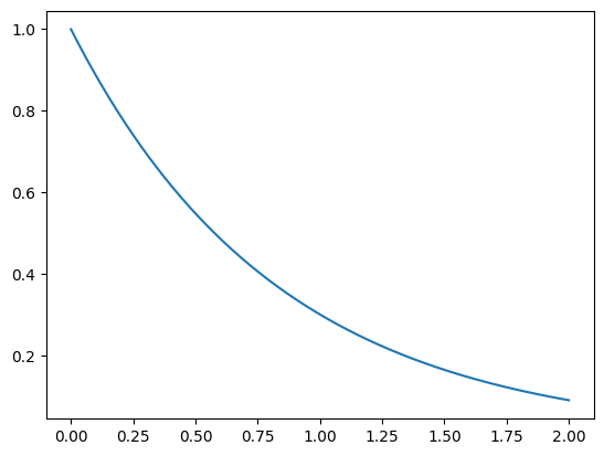
fcn = lambda t,y,a: -a*y
ts = torch.linspace(0, 2, 1000, requires_grad=True)
a = torch.tensor(1.2, requires_grad=True)
y0 = torch.tensor(1.0, requires_grad=True)
yt = solve_ivp(fcn, ts, y0, params=(a,), method=euler_forward)  # custom implementation
_ = plt.plot(ts.detach(), yt.detach())  # y(t) = exp(-a*t)

Although the implementation is written without gradient propagation, xitorch can still propagate the gradient. This is because xitorch uses analytical expression for the backward instead of propagating the gradient through a specific implementation.

# first order grad
grad_a, = torch.autograd.grad(yt[-1], a, create_graph=True)
grad_a_true = -ts[-1] * torch.exp(-a*ts[-1])  # dy/da = -t*exp(-a*t)
print(grad_a.data, grad_a_true.data)

tensor(-0.1809) tensor(-0.1814)

# second order grad
grad_a2, = torch.autograd.grad(grad_a, a)
grad_a2_true = ts[-1]**2 * torch.exp(-a*ts[-1])  # d2y/da2 = t*t*exp(-a*t)
print(grad_a2.data, grad_a2_true.data)

tensor(0.3618) tensor(0.3629)

We can see that with custom implementation (which does not propagate gradient), it can still calculate the first and second order gradients. The small discrepancy above is due to the imperfect calculation of Euler forward method.